Spectral extraction from a singe order transit timeseries data

In the present notebook, we will extract spectra from a single order transit timeseries data. We will use WASP-39 transit timeseries data obtained with NIRCam/JWST for Transiting Exoplanet Community Early Release Science (ERS) program. All data products can be found on the MAST portal: this contains raw uncalibrated data (files with uncal.fits extension), calibrated data (rateints.fits and calints.fits) and even spectrum timeseries data (x1dints.fits). Here we will use rateints.fits files to extract spectrum (see, the documentation of the jwst pipeline to know more). We downloaded all files and put them in the same directory as this notebook.

We first need to “correct” this data for NaN values, 0s and cosmic rays, which will be our first task. We can then perform a background subtraction. Finally we will extract a spectrum timeseries from this dataset.

import numpy as np
import matplotlib.pyplot as plt
import os
from stark import SingleOrderPSF, optimal_extract, reduce
from astropy.stats import mad_std
from glob import glob
from astropy.io import fits
from tqdm import tqdm
from path import Path
from scipy.optimize import curve_fit as cft
from mpl_toolkits.axes_grid1 import make_axes_locatable
import warnings

Loading the dataset

Since the data volume is too big, the data products are delievered in segments. For WASP-39 NIRCam data, there are 4 segments. We first load data in all 4 segments and put them in a single numpy array below. The data in each segment contains several hundreads of individual exposures, or, frames. Each frame has a data array, an error array, a dq (data quality, i.e., bad-pixel map) array and a time array. We will extract all 4 types of information from each frame.

visit = 'NRCLW'

# Input and Output paths
p1 = os.getcwd()
if not Path(p1 + '/Figures').exists():
    os.mkdir(p1 + '/Figures')

## Segments!!!
segs = ['00' + str(i+1) for i in range(4)]

# For 1st segment
## Loading the .fits file
fhdul = glob(p1 + '/*seg001_nrcalong_rateints.fits')[0]
hdul = fits.open(fhdul)
## 1, 2 and 3rd products are data, errors and bad-pixel map, respectively
raw_data, raw_err, dq, time_bjd = hdul[1].data, hdul[2].data, hdul[3].data, hdul[4].data['int_mid_BJD_TDB']
## All values >0 in bad pixel maps are "bad"; we create a simpler bad-pixel map here,
# 0 means bad pixel and 1 means a good pixel (the same convention used by stark)
mask = np.ones(dq.shape)
mask[dq > 0] = 0.

# Repeating the same for the other segments
for i in range(len(segs)-1):
    fhdul = glob(p1 + '/*seg' + segs[i+1] + '_nrcalong_rateints.fits')[0]
    hdul = fits.open(fhdul)
    # Data
    raw_data = np.vstack((raw_data, hdul[1].data))
    # Errors
    raw_err = np.vstack((raw_err, hdul[2].data))
    # DQ
    dq, m1 = hdul[3].data, np.ones(hdul[1].data.shape)
    m1[dq>0] = 0.
    mask = np.vstack((mask, m1))
    # Times
    time_bjd = np.hstack((time_bjd, hdul[4].data['int_mid_BJD_TDB']))

time_bjd = time_bjd + 2400000.5
nint = np.random.randint(0, raw_data.shape[0])

Correcting the dataset

Although the data that we gathered above is a calibrated data, we still need to perform additional checks to this dataset, looking for 0s and NaN, for instance. 0s and NaN values in error arrays will specially be painful since we aim to use error array as weighting while fitting a PSF. So, let’s first correct for 0s and NaN from the error array. We will, additionally, consider these pixels as “bad” and add them to the default bad-pixel map.

## Correct errorbars
print('>>>> --- Correcting errorbars (for zeros and NaNs)...')
med_err = np.nanmedian(raw_err.flatten())
## Changing Nan's and zeros in error array with median error
corr_err1 = np.copy(raw_err)
corr_err2 = np.where(raw_err != 0., corr_err1, med_err)
corrected_errs = np.where(np.isnan(raw_err) != True, corr_err2, med_err)
print('>>>> --- Done!!')

print('>>>> --- Updating the bad-pixel map...')
## Making a bad-pixel map (1s are good pixels, 0s are bad pixels)
mask_bp1 = np.ones(raw_data.shape)
mask_bp2 = np.where(raw_err != 0., mask_bp1, 0.)               # This will place 0 in mask where errorbar == 0
mask_bp3 = np.where(np.isnan(raw_err) != True, mask_bp2, 0.)   # This will place 0 in mask where errorbar is Nan
mask_badpix = mask * mask_bp3     # Adding those pixels which are identified as bad by the pipeline (and hence 0)
print('>>>> --- Done!!')

>>>> --- Correcting errorbars (for zeros and NaNs)...
>>>> --- Done!!
>>>> --- Updating the bad-pixel map...
>>>> --- Done!!

Our data will be contaminated with a lot of cosmic rays, we want to identify those pixels and add them to our bad pixel map. Our method of identifying cosmic rays is pretty simple: we will generate a median dataframe, and compare this median frame with all frames. Since cosmic rays are outliers, we should be able to identify them by comparing each frame with a median frame. We further want to correct these values by taking mean of neighbouring pixels.

def identify_crays(frames, mask_bp, clip=5, niters=5):
    """Given a data cube and bad-pixel map, this function identifies cosmic rays by using median frame"""
    # Masking bad pixels as NaN
    mask_cr = np.copy(mask_bp)
    for _ in range(niters):
        # Flagging bad data as Nan
        frame_new = np.copy(frames)
        frame_new[mask_cr == 0.] = np.nan
        # Median frame
        with warnings.catch_warnings():
            warnings.simplefilter('ignore', RuntimeWarning)
            median_frame = np.nanmedian(frame_new, axis=0)  # 2D frame
            # Creating residuals
            resids = frame_new - median_frame[None,:,:]
            # Median and std of residuals
            med_resid, std_resid = np.nanmedian(resids, axis=0), np.nanstd(resids, axis=0)
        limit = med_resid + (clip*std_resid)
        mask_cr1 = np.abs(resids) < limit[None,:,:]
        mask_cr = mask_cr1*mask_bp
    return mask_cr

def replace_nan(data, max_iter = 50):
    """Replaces NaN-entries by mean of neighbours.
    Iterates until all NaN-entries are replaced or
    max_iter is reached. Works on N-dimensional arrays.
    """
    nan_data = data.copy()
    shape = np.append([2*data.ndim], data.shape)
    interp_cube = np.zeros(shape)
    axis = tuple(range(data.ndim))
    shift0 = np.zeros(data.ndim, int)
    shift0[0] = 1
    shift = []     # Shift list will be [(-1, 0), (1, 0), (0, -1), (0, 1)]
    for n in range(data.ndim):
        shift.append(tuple(np.roll(-shift0, n)))
        shift.append(tuple(np.roll(shift0, n)))
    for _j in range(max_iter):
        for n in range(2*data.ndim):
            interp_cube[n] = np.roll(nan_data, shift[n], axis = axis)   # interp_cube would be (4, data.shape[0], data.shape[1]) sized array
        with warnings.catch_warnings():                                 # with shifted position in each element (so that we can take its mean)
            warnings.simplefilter('ignore', RuntimeWarning)
            mean_data = np.nanmean(interp_cube, axis=0)
        nan_data[np.isnan(nan_data)] = mean_data[np.isnan(nan_data)]
        if np.sum(np.isnan(nan_data)) == 0:
            break
    return nan_data

## Mask with cosmic rays
### Essentially this mask will add 0s in the places of bad pixels...
print('>>>> --- Identifying cosmic rays and updating the bad-pixel map...')
mask_bcr = identify_crays(raw_data, mask_badpix)
print('Total per cent of masked points:\
    {:.4f} %'.format(100 * (1 - np.sum(mask_bcr) / (mask_bcr.shape[0] * mask_bcr.shape[1] * mask_bcr.shape[2]))))
print('>>>> --- Done!!')

# And interpolating the data in bad-pixels with mean of neighbouring pixels
print('>>>> --- Correcting data...')
corrected_data_wo_bkg = np.copy(raw_data)
corrected_data_wo_bkg[mask_bcr == 0] = np.nan
for i in range(corrected_data_wo_bkg.shape[0]):
    corrected_data_wo_bkg[i,:,:] = replace_nan(corrected_data_wo_bkg[i,:,:])
print('>>>> --- Done!!')

>>>> --- Identifying cosmic rays and updating the bad-pixel map...
Total per cent of masked points:      5.4090 %
>>>> --- Done!!
>>>> --- Correcting data...
>>>> --- Done!!

Let’s now visualise our data – we will display one randomly selected frame below:

plt.figure(figsize=(15,5))
plt.imshow(corrected_data_wo_bkg[nint,4:,:], interpolation='none', aspect='auto')
plt.title('Example data frame')

It looks good! So, there are 256 rows (spatial direction) and 2048 columns (dispersion direction). The location of the trace is clearly seen. Let’s plot the value of flux for a given column:

plt.figure(figsize=(15,5))
plt.plot(corrected_data_wo_bkg[nint,:,500])
plt.ylim([-2.5,2.5])
plt.axhline(0., color='k')
plt.xlabel('Row number')
plt.ylabel('Counts')
plt.title('Flux level in an arbitrary column of an arbitrary integration')

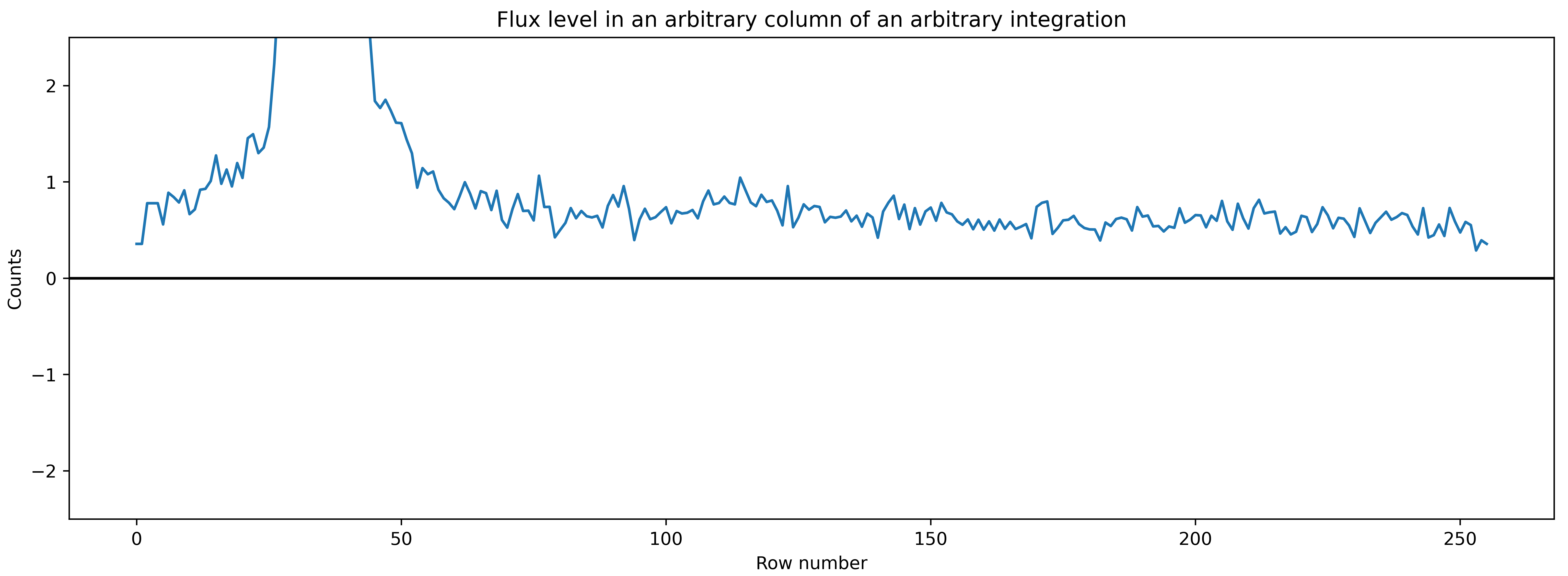
It is evident that the flux values in the background are not exactly zero. So, we need to perform a background subtraction.

Background subtraction

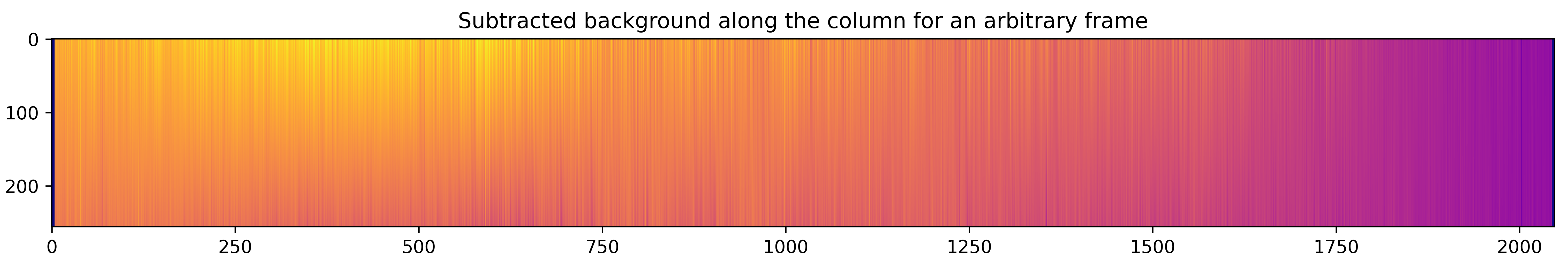
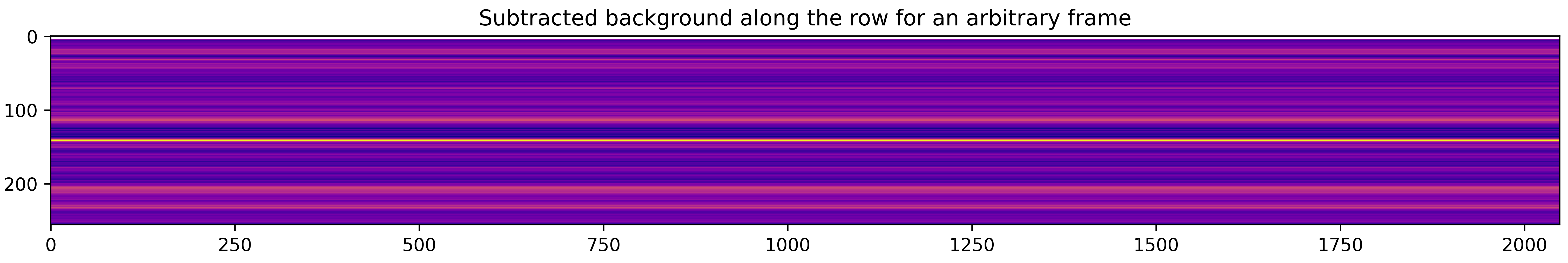
We will perform background subtraction in both column and row direction. stark has functions to do this. Along the column, we will fit a linear polynomial to the background pixels for each column and then subtract the estimated background from each pixels. On the other hand, we will simply take median of background pixels along the row direction to estimate the background and then subtract that value from all pixels along the row.

We need to define the background region for that. Roughly looking at example data frame above, all rows above 80th row and 1750th column are basically background. So, we will define our mask in such a way:

msk_bkg = np.ones(corrected_data_wo_bkg[nint,:,:].shape)
msk_bkg[0:80,0:1750] = 0.

plt.figure(figsize=(15,5))
plt.imshow(msk_bkg, interpolation='none')
plt.title('Background mask')

And, below we do background subtraction using :code:`stark` functions stark.reduce.polynomial_bkg_cols (for a background subtraction along columns) and stark.reduce.row_by_row_bkg_sub (along the row).

corrected_data_bkg = np.ones(corrected_data_wo_bkg.shape)
sub_bkg_col = np.ones(corrected_data_wo_bkg.shape)
for i in tqdm(range(corrected_data_wo_bkg.shape[0])):
    corrected_data_bkg[i,:,:], sub_bkg_col[i,:,:] =\
        reduce.polynomial_bkg_cols(corrected_data_wo_bkg[i,:,:], mask=msk_bkg*mask_bcr[i,:,:], deg=1, sigma=5)

corrected_data = np.ones(corrected_data_wo_bkg.shape)
sub_bkg_row = np.ones((corrected_data_wo_bkg.shape[0], corrected_data_wo_bkg.shape[1]))
for i in tqdm(range(corrected_data.shape[0])):
    corrected_data[i,:,:], sub_bkg_row[i,:] = \
        reduce.row_by_row_bkg_sub(corrected_data_bkg[i,:,:], mask=msk_bkg*mask_bcr[i,:,:])

plt.figure(figsize=(15,5))
plt.imshow(sub_bkg_col[nint,:,:], cmap='plasma', interpolation='none')
plt.title('Subtracted background along the column for an arbitrary frame')

plt.figure(figsize=(15,5))
plt.imshow(sub_bkg_row[nint,:,None] * np.ones(corrected_data[nint,:,:].shape), cmap='plasma', interpolation='none')
plt.title('Subtracted background along the row for an arbitrary frame')

Tracing the spectra

The first step of the spectral extraction is to find the trace positions – we will use center-of-flux method to find location of spectral trace at each wavelength column for every time integration.

def quadratic(x, a, b, c):
    return a*(x**2) + b*x + c

def jitter(x, jit):
    return x + jit

# Finding trace
def trace_pos(data, xstart, xend, ystart, yend):
    """Given a data frame and starting location, this function will find trace using centre-of-flux method"""
    xpos = np.arange(xstart, xend, 1)
    rough_trace = np.zeros((data.shape[0], len(xpos)))
    for i in tqdm(range(data.shape[0])):
        frame = data[i,:,:]
        row = np.arange(frame.shape[0])
        centre = np.sum(frame[ystart:yend,:]*row[ystart:yend, None], axis=0) / \
            np.maximum(np.sum(frame[ystart:yend,:], axis=0), 1)
        rough_trace[i,:] = centre[xstart:xend]
    median_rough_trace = np.nanmedian(rough_trace, axis=0)
    # Fitting a quadratic function to this
    popt, pcov = cft(quadratic, xpos, median_rough_trace)
    median_trace = quadratic(xpos, *popt)
    # And we will now fit jitter to each integration
    dx = np.zeros(data.shape[0])
    for i in tqdm(range(data.shape[0])):
        popt, _ = cft(jitter, rough_trace[i,:], median_trace)
        dx[i] = popt[0]
    return xpos, median_trace, dx

xpos, trace1, dx1 = trace_pos(corrected_data[:,4:,:], 40, 1600, 25, 35)
ypos2d = np.zeros((corrected_data.shape[0], len(xpos)))
for i in range(ypos2d.shape[0]):
    ypos2d[i,:] = trace1 + dx1[i]

plt.figure(figsize=(15,5))
plt.imshow(corrected_data[nint,4:,:], interpolation='none', aspect='auto')
plt.plot(xpos, trace1, 'k-')
plt.ylim([50,0])
plt.title('Example data with the location of spectral trace')

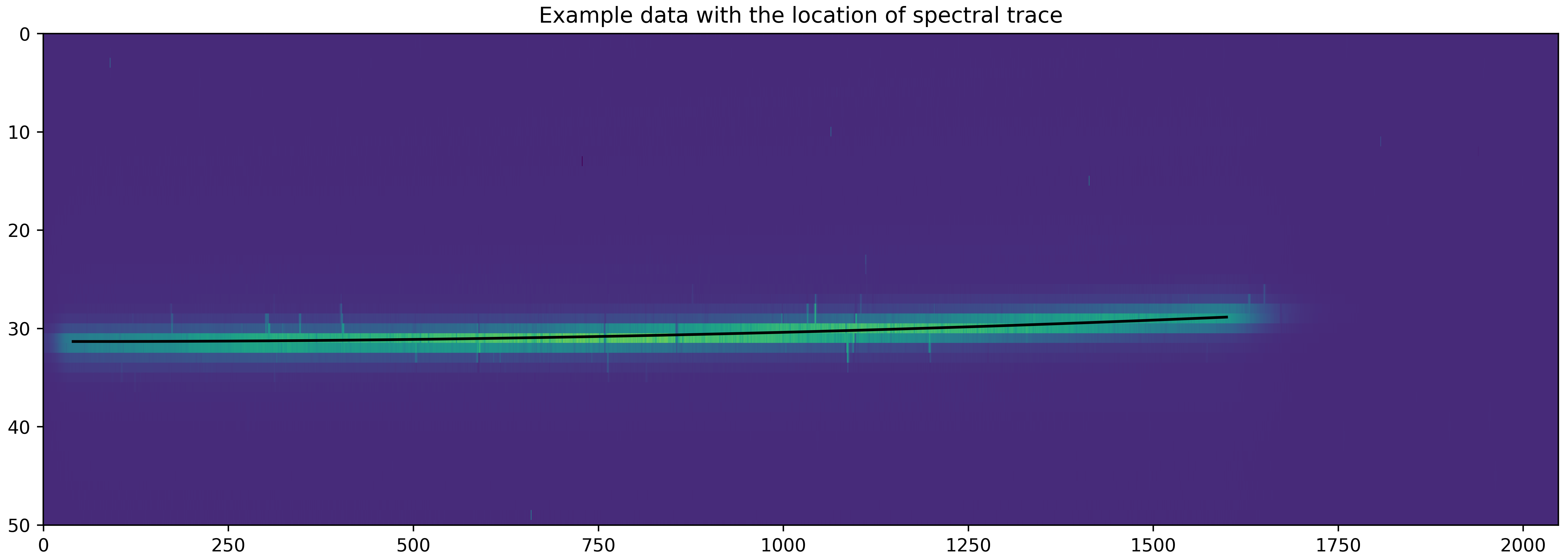
What we plot above is the median trace location – on the top of this there should be a jitter of trace as a function of time. Let’s plot that jitter below:

plt.figure(figsize=(15,5))
plt.plot(np.arange(len(dx1)), dx1, 'k-')
plt.xlabel('Integration number')
plt.ylim([-0.007, 0.007])
plt.ylabel('Jitter')

The trace looks more or less stable, the average jitter is at around 0.004 pixels – that is very good! So, we will use these trace positions to identify the location of trace on data.

Initial estimate of PSF

We mentioned above that while PSF would not change with time, it will change significantly with wavelength. So, we want to fit a 2D spline to get a robust estimate of PSF. However, before doing that, let’s approximate that the PSF doesn’t change with wavelength. This assumption can give us a first rough estimate of stellar spectra which we can use as normalisation constant in next step.

So, let’s fit 1D spline to the data as a function of spatial coordinate, i.e., distance from trace. In stark we first create a stark data object using SingleOrderPSF class which will load data. This class will take the data, variance, masked pixels, aperture half-widths and trace locations as inputs. Note that the SingleOrderPSF takes 3D arrays as data, variance and masked pixels with dimensions of (nFrames, nRows, nCols) assuming the trace run along the row. Similarly trace locations are a 2D array giving trace positions for each integration (nFrames, TraceLocations).

Once we load the data, we can fit a 1D spline using univariate_psf_frame method, which will return PSF frame and best-fitted spline object.

data1d = SingleOrderPSF(frame=corrected_data[:,4:,xpos[0]:xpos[-1]+1],\
                        variance=corrected_errs[:,4:,xpos[0]:xpos[-1]+1]**2,\
                        ord_pos=ypos2d, ap_rad=9., mask=mask_bcr[:,4:,xpos[0]:xpos[-1]+1])
psf_frame1d, psf_spline1d, _ = data1d.univariate_psf_frame(niters=3, oversample=2, clip=10000)

# Details of the data, in form of a pixel table (see, API) is stored in data.norm_array
ts1 = np.linspace(np.min(data1d.norm_array[:,0]), np.max(data1d.norm_array[:,0]), 1000)
msk1 = np.asarray(data1d.norm_array[:,4], dtype=bool)
plt.figure(figsize=(16/1.5, 9/1.5))
plt.errorbar(data1d.norm_array[msk1,0], data1d.norm_array[msk1,1], fmt='.')
plt.plot(ts1, psf_spline1d(ts1), c='k', lw=2., zorder=10)
plt.xlabel('Distance from the trace')
plt.ylabel('Normalised flux')
plt.savefig('1dspline.png', dpi=500)

Iter 1 / 3: 1.90234 per cent masked.
Iter 2 / 3: 1.90234 per cent masked.
Iter 3 / 3: 1.90234 per cent masked.

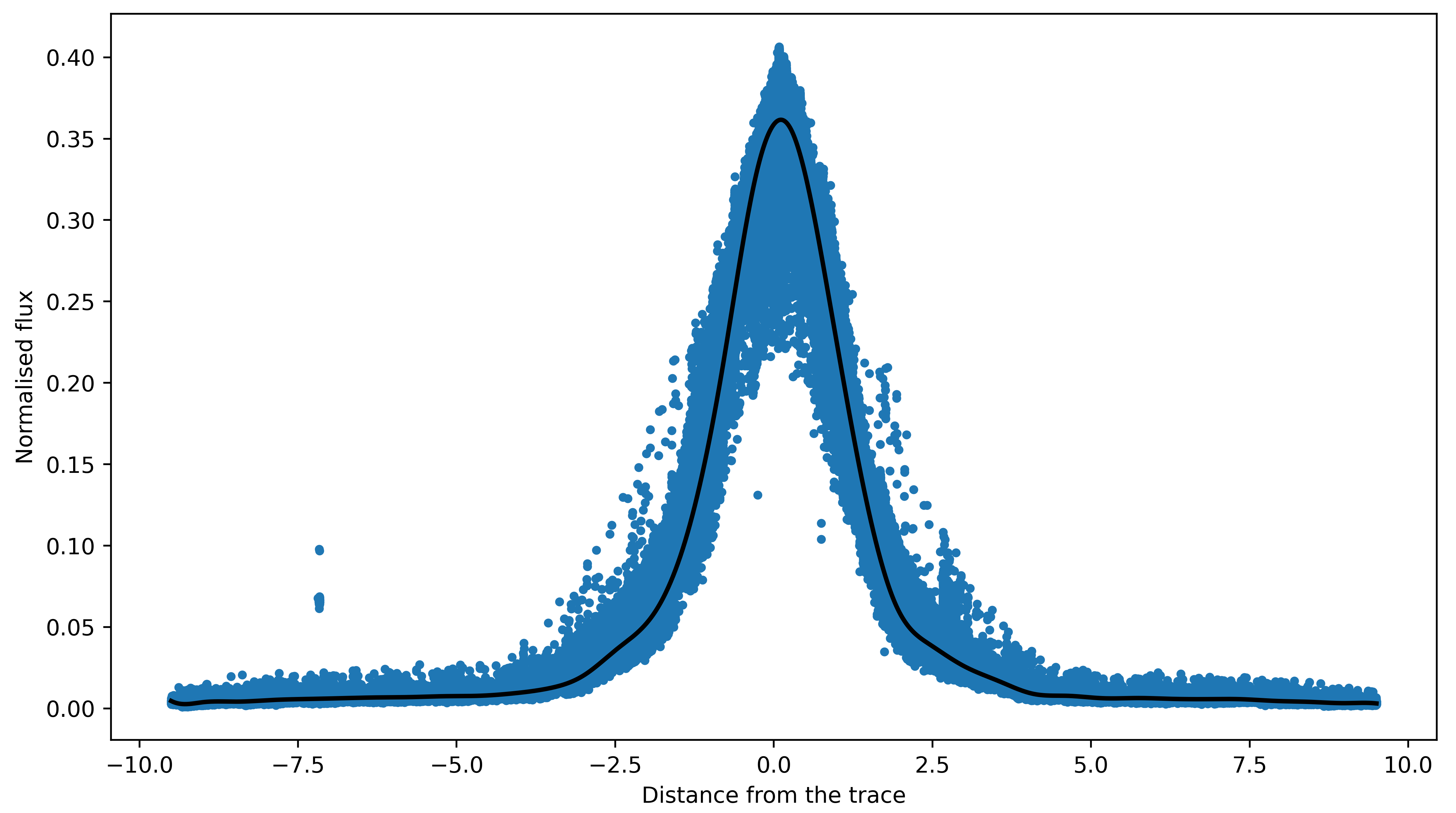
Nice! Above plot shows all data points (in blue) as a function of distance from trace and black line is the best-fitted PSF. As a first estimate this is looking very good. Let’s now use this PSF to find t imeseries of stellar spectra using optimal_extract function.

(The third return variable which we did not save above while doing data1.univariate_psf_frame is updated mask returned by the function. When we fit a spline to the data, it will identify outliers points beyond our preferred clipping limit – clip argument – and add them to the mask. Along with the PSF frame and the spline object, univariate_psf_frame (and also the bivariate_psf_frame, see below) functions will return this mask in form of pixel table. Users can use data1d.table2frame function to get back a 2D updated mask.

This type of sigma clipping is usually useful to identify cosmic rays. In this example, however, we used a different method to identify cosmic rays (see, above), so we do not need to perform a sigma clipping here again. That is why we used clip=10000 to essentially perform no sigma clipping. See, Tutorial 2 for more information on this.)

spec1d, var1d = np.zeros((psf_frame1d.shape[0], psf_frame1d.shape[2])), np.zeros((psf_frame1d.shape[0], psf_frame1d.shape[2]))
syth1d = np.zeros(psf_frame1d.shape)
for inte in tqdm(range(spec1d.shape[0])):
    spec1d[inte,:], var1d[inte,:], syth1d[inte,:,:] = optimal_extract(psf_frame=psf_frame1d[inte,:,:],\
                                                                      data=corrected_data[inte,4:,xpos[0]:xpos[-1]+1],\
                                                                      variance=corrected_errs[inte,4:,xpos[0]:xpos[-1]+1]**2,\
                                                                      mask=mask_bcr[inte,4:,xpos[0]:xpos[-1]+1],\
                                                                      ord_pos=ypos2d[inte,:], ap_rad=9.)

We now have a first estimate of timeseries of stellar spectra. We can use this as a normalising spectra in the next step.

Robust estimate of PSF

As already mentioned, while PSF doesn’t change much with time, it does change with wavelength. So, our above approximation of assuming a constant PSF with wavelength was not good. To take care of this, we will now assume that PSF changes with wavelength and we will fit a 2D spline to the data as a function of spatial direction and wavelength. To do so, we will first load the data as previously, but now we will provide initial estimate of spectra to use it as a normalising constant.

After loading the data we will use bivariate_psf_frame method to fit 2D spline to this data:

data2 = SingleOrderPSF(frame=corrected_data[:,4:,xpos[0]:xpos[-1]+1],\
                       variance=corrected_errs[:,4:,xpos[0]:xpos[-1]+1]**2,\
                       ord_pos=ypos2d, ap_rad=9., mask=mask_bcr[:,4:,xpos[0]:xpos[-1]+1],\
                       spec=spec1d)
psf_frame2d, psf_spline2d = data2.bivariate_psf_frame(niters=3, oversample=2, knot_col=10, clip=10000)

/Users/japa6985/opt/anaconda3/envs/jwst/lib/python3.9/site-packages/scipy/interpolate/fitpack2.py:1272: UserWarning:
The coefficients of the spline returned have been computed as the
minimal norm least-squares solution of a (numerically) rank deficient
system (deficiency=55). If deficiency is large, the results may be
inaccurate. Deficiency may strongly depend on the value of eps.
warnings.warn(message)
Iter 1 / 3: 1.90234 per cent masked.
Iter 2 / 3: 1.90234 per cent masked.
Iter 3 / 3: 1.90234 per cent masked.

Before finding the time-series of spectra, let’s see how we well we fit the splines. For this, we will visualise data and fitted splines for one given colum.

# Details are not that important:
# But what we are trying to do below is to find data from an arbitrary column for _all_ integration
# And then we will see how the fitted 2D spline behaves to this data

ncol1 = np.random.choice(xpos)  # Arbitrary column number
msk5 = data2.col_array_pos[:,ncol1,0]     # Mask data
npix1 = data2.col_array_pos[:,ncol1,1]    # Pixel radius data

xpoints = np.array([])     # To save x (pixel coordinate), y (column no), z (flux)
ypoints = np.array([])
zpoints = np.array([])
for i in range(len(msk5)):
    xdts = data2.norm_array[msk5[i]:msk5[i]+npix1[i],0]
    ydts = data2.norm_array[msk5[i]:msk5[i]+npix1[i],3]
    zdts = data2.norm_array[msk5[i]:msk5[i]+npix1[i],1]
    msk_bad = np.asarray(data2.norm_array[msk5[i]:msk5[i]+npix1[i],4], dtype=bool)
    xdts, ydts, zdts = xdts[msk_bad], ydts[msk_bad], zdts[msk_bad]
    xpoints = np.hstack((xpoints, xdts))
    ypoints = np.hstack((ypoints, ydts))
    zpoints = np.hstack((zpoints, zdts))

# Creating a continuous grid of points
xpts1 = np.linspace(np.min(xpoints)-0.1, np.max(xpoints)+0.1, 1000)
ypts1 = np.ones(1000)*ypoints[0]

fits_2d = psf_spline2d(xpts1, ypts1, grid=False)

plt.figure(figsize=(16/1.5,9/1.5))
plt.errorbar(xpoints, zpoints, fmt='.')
plt.plot(xpts1, fits_2d, 'k-')
plt.plot(xpoints, psf_spline2d(xpoints, ypoints, grid=False), 'k.')
plt.axvline(0., color='k', ls='--')
plt.title('All frames, for Column ' + str(ncol1))
plt.xlabel('Distance from the trace')
plt.ylabel('Normalised flux')

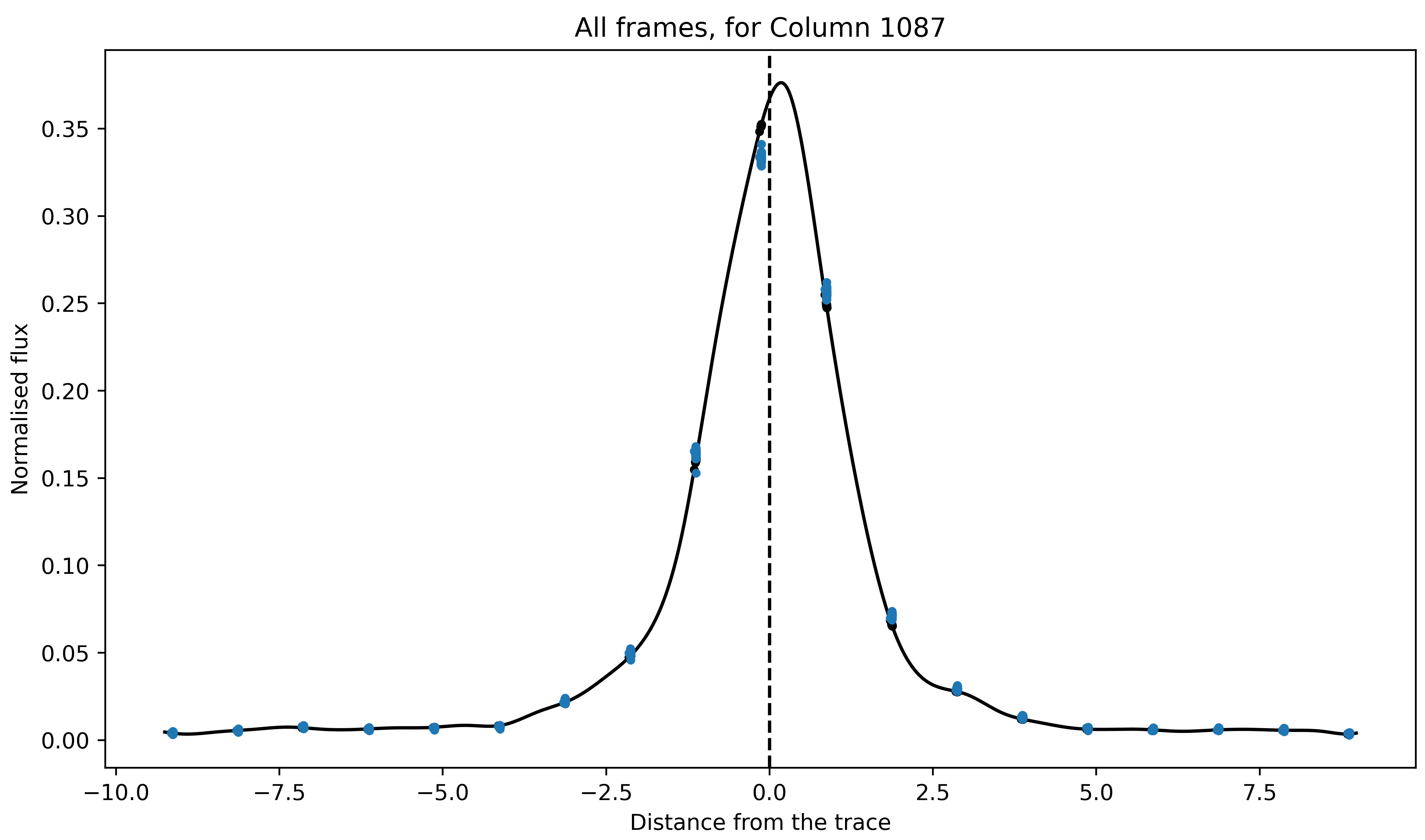
The blue and black (barely visible) points are original data points and their estimated value based on the best fitted spline (black line). The fitted spline is slightly asymmetric but that is okay. Overall, we did a good job.

Now, we mentioned that the main reason to use 2D splines was that the PSF was not constant as a function of wavelength. So, let’s now see how PSF (i.e., its amplitude and FWHM) changes with wavelength.

# Defining pixel coordinates
pix_cor_res = 50000
pix_corr = np.linspace(-8., 8., pix_cor_res)

cols = xpos - xpos[0]
max_amp = np.zeros(len(cols))
fwhm = np.zeros(len(cols))

for i in range(len(cols)):
    fit2 = psf_spline2d(x=pix_corr, y=np.ones(pix_cor_res)*cols[i], grid=False)
    # Maximum amplitude
    max_amp[i] = np.max(fit2)
    # Maximum amplitude location
    idx_max_amp = np.where(fit2 == np.max(fit2))[0][0]
    # fwhm
    hm = (np.max(fit2) + np.min(fit2))/2
    idx_hm = np.where(np.abs(fit2 - hm)<0.005)[0]
    idx_hm_up, idx_hm_lo = 0, 0
    diff_up1, diff_lo1 = 10., 10.
    for j in range(len(idx_hm)):
        if idx_hm[j] > idx_max_amp:
            diff_u1 = np.abs(fit2[idx_hm[j]] - hm)
            if diff_u1 < diff_up1:
                diff_up1 = diff_u1
                idx_hm_up = idx_hm[j]
        else:
            diff_l1 = np.abs(fit2[idx_hm[j]] - hm)
            if diff_l1 < diff_lo1:
                diff_lo1 = diff_l1
                idx_hm_lo = idx_hm[j]
    fwhm[i] = np.abs(pix_corr[idx_hm_up] - pix_corr[idx_hm_lo])

fig, axs = plt.subplots(2, 1, figsize=(15, 5), sharex=True, facecolor='white')

axs[0].plot(xpos, max_amp, 'k-')
axs[0].set_ylabel('Maximum Amplitude', fontsize=14)

axs[1].plot(xpos, fwhm, 'k-')
axs[1].set_ylabel('FWHM', fontsize=14)
axs[1].set_xlabel('Column number', fontsize=14)

axs[1].set_xlim([xpos[0], xpos[-1]])

axs[0].set_title('PSF evolution with wavelength', fontsize=15)

plt.setp(axs[0].get_yticklabels(), fontsize=12)
plt.setp(axs[1].get_xticklabels(), fontsize=12)
plt.setp(axs[1].get_yticklabels(), fontsize=12)

plt.tight_layout()

Both the amplitude and FWHM is a bit wiggly. This maybe because we used oversample=2 while fitting the 2D spline. When we do this, we put 2 times more knots in the spatial direction, and this could make PSF more noisy (or, more wiggly). One can use oversample=1 (the default option) which would put 1 knot per pixel – while this could “stablise” the PSF, its fitting to the data will not be as good. Ideally, one should use oversample=1 and then repeat this whole procedure iteratively. But, for our purposes, using oversample=2 is okay.

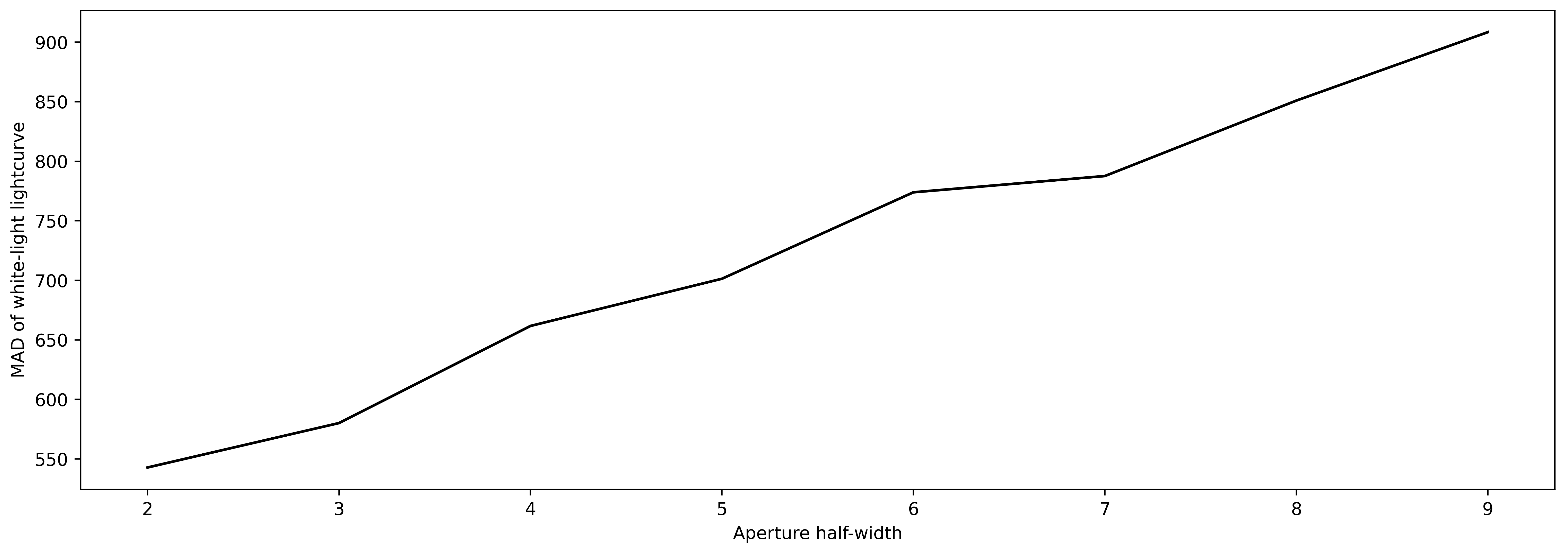
Aperture half-width selection

Now, we want to use this PSF to extract the stellar spectra. Until now, we were using aperture half-width of 9 pixels to fit the splines and to extract the spectra. And that is totally fine. However, it could be possible that by changing the aperture half-width one could get a lower scatter in the final white-light lightcurve. So, what we will do below is to extract spectra for a series of aperture half-widths from 2 to 9 pixels. After spectral extraction we will compute a white-light lightcurve by taking weighted average of all spectroscopic lightcurves (i.e., flux as a function of time for each wavelengths). Finally, we will compute the MAD of this lightcurve and compare it with MAD value of white-light lightcurves found with different apertures. We will select the aperture with minimum MAD on white-light lightcurve.

apertures = np.arange(2,10,1)
scatter = np.zeros(len(apertures))

for aps in range(len(apertures)):
    spec1d, var1d = np.zeros((psf_frame2d.shape[0], psf_frame2d.shape[2])), np.zeros((psf_frame2d.shape[0], psf_frame2d.shape[2]))
    syth1d = np.zeros(psf_frame2d.shape)
    for inte in tqdm(range(spec1d.shape[0])):
        spec1d[inte,:], var1d[inte,:], syth1d[inte,:,:] = optimal_extract(psf_frame=psf_frame2d[inte,:,:],\
                                                                        data=corrected_data[inte,4:,xpos[0]:xpos[-1]+1],\
                                                                        variance=corrected_errs[inte,4:,xpos[0]:xpos[-1]+1]**2,\
                                                                        mask=mask_bcr[inte,4:,xpos[0]:xpos[-1]+1],\
                                                                        ord_pos=ypos2d[inte,:], ap_rad=apertures[aps])
    # Computing white-light lightcurve
    wht_lc = np.nansum(spec1d/var1d, axis=1) / np.nansum(1/var1d, axis=1)
    # And its scatter
    scatter[aps] = mad_std(wht_lc/np.nanmedian(wht_lc)) * 1e6

plt.figure(figsize=(15,5))
plt.plot(apertures, scatter, 'k-')
plt.xlabel('Aperture half-width')
plt.ylabel('MAD of white-light lightcurve')

Optimal extraction of the spectral timeseries

Perfect! We now have an optimal aperture size. We will use this aperture size to extract spectra again:

min_scat_ap = apertures[np.argmin(scatter)]

spec1d, var1d = np.zeros((psf_frame2d.shape[0], psf_frame2d.shape[2])), np.zeros((psf_frame2d.shape[0], psf_frame2d.shape[2]))
syth1d = np.zeros(psf_frame2d.shape)
for inte in tqdm(range(spec1d.shape[0])):
    spec1d[inte,:], var1d[inte,:], syth1d[inte,:,:] = optimal_extract(psf_frame=psf_frame2d[inte,:,:],\
                                                                      data=corrected_data[inte,4:,xpos[0]:xpos[-1]+1],\
                                                                      variance=corrected_errs[inte,4:,xpos[0]:xpos[-1]+1]**2,\
                                                                      mask=mask_bcr[inte,4:,xpos[0]:xpos[-1]+1],\
                                                                      ord_pos=ypos2d[inte,:], ap_rad=min_scat_ap)

Let’s plot all spectra (or, spectral timeseries) on the top of each other:

plt.figure(figsize=(15,5))
for i in range(spec1d.shape[0]):
    plt.plot(xpos, spec1d[i,:], 'k', alpha=0.1)
plt.xlabel('Column number')
plt.ylabel('#')
plt.title('Timeseries of spectra')

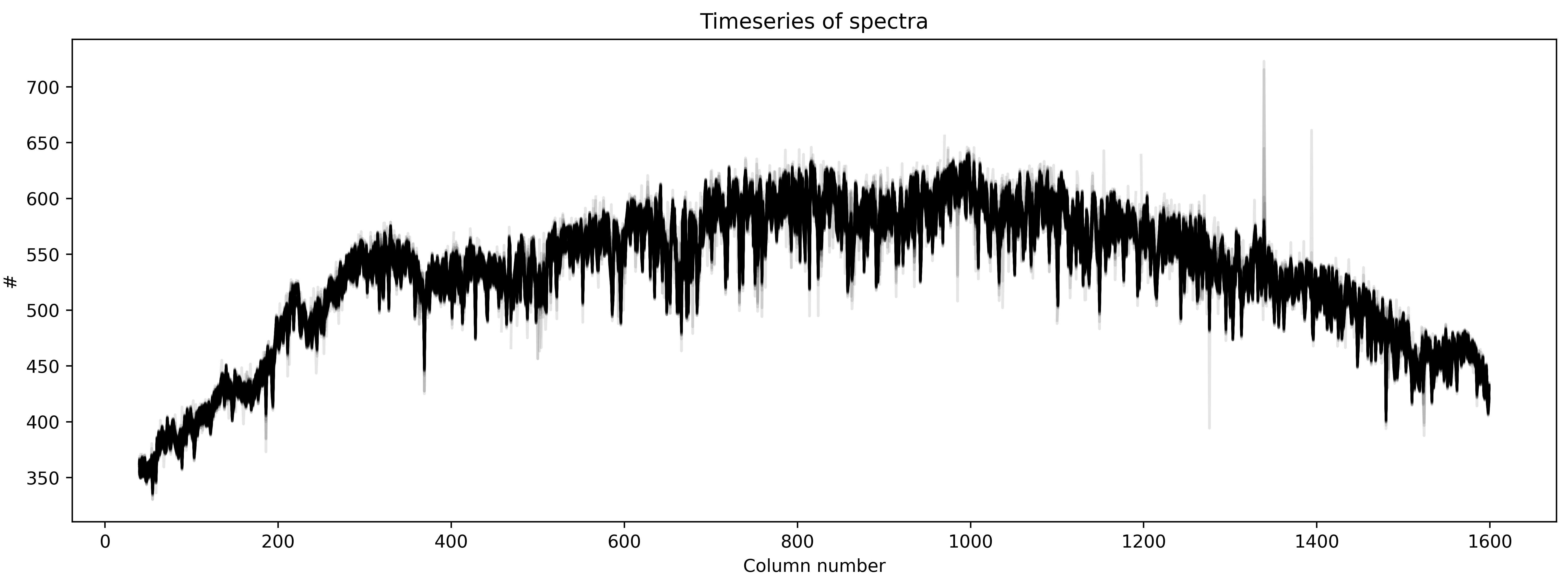
Good! The scatter (or the width) that we see above is because the level of flux changes during the transit event.

Residual frame

When we fit 2D spline to the data, we are basically modelling the trace. So, in principle, we do spectral extraction, we should have a synthetic model of the data. Indeed, we were saving this model for each time when we performed spectral extraction using optimal_extract function. We can subtract this sythetic model from our dataset to find what is called residual frame. Ideally, this frame should look like a white-noise. If not there is some left-over noise in the data or spline fitting was not perfect.

In any case the median residual frame should show us the static leftover noise that was not fitted. If one find any such noise one can subtract this median residual frame from our original data and repeat the whole procedure of spline fitting until there remains only white noise in the median residual frame.

So, now, let’s see how the median residual frame looks like:

resid1 = np.zeros(syth1d.shape)
for j in range(resid1.shape[0]):
    resid1[j,:,:] = corrected_data[j,4:,xpos[0]:xpos[-1]+1] - syth1d[j,:,:]

med_resid = np.nanmedian(resid1, axis=0)

plt.figure(figsize=(15,5))
im = plt.imshow(med_resid, interpolation='none')#, aspect='auto')
im.set_clim([-5,5])
plt.xlim([0,315])
plt.ylim([20,40])
plt.title('Median residual frame')

plt.figure(figsize=(15,5))
im = plt.imshow(med_resid, interpolation='none')#, aspect='auto')
im.set_clim([-5,5])
plt.xlim([315,2*315])
plt.ylim([20,40])

plt.figure(figsize=(15,5))
im = plt.imshow(med_resid, interpolation='none')#, aspect='auto')
im.set_clim([-5,5])
plt.xlim([2*315, 3*315])
plt.ylim([20,40])

plt.figure(figsize=(15,5))
im = plt.imshow(med_resid, interpolation='none')#, aspect='auto')
im.set_clim([-5,5])
plt.xlim([3*315, 4*315])
plt.ylim([20,40])

plt.figure(figsize=(15,5))
im = plt.imshow(med_resid, interpolation='none')#, aspect='auto')
im.set_clim([-5,5])
plt.xlim([4*315, 5*315])
plt.ylim([20,40])

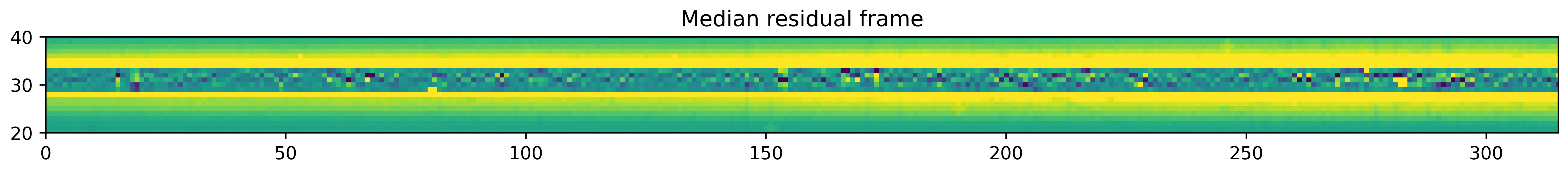
Ahh good! Maybe there is some structure in these image – but for the purpose of this analysis, we can safely assume that this is just some white-noise. Interested reader can subtract this median residual image from each dataframe and repeat the whole procedure of spline fitting again. That would definately remove any leftover static noise.

Lightcurves

Now, we will compute white-light lightcurve by taking a weighted average of spectroscopic lightcurves (i.e., timeseries of flux at each wavelength).

wht_light_lc = np.nansum(spec1d/var1d, axis=1) / np.nansum(1/var1d, axis=1)
wht_light_err = 1/np.sqrt(np.nansum(1/var1d, axis=1))

plt.figure(figsize=(15,5))
plt.errorbar(time_bjd, wht_light_lc/np.nanmedian(wht_light_lc), \
            yerr=wht_light_err/np.nanmedian(wht_light_lc), fmt='.', c='k')
plt.title('White-light lightcurve, MAD: {:.4f} ppm'.format(mad_std(wht_light_lc/np.nanmedian(wht_light_lc)) * 1e6))
plt.xlabel('Time (BJD)')
plt.ylabel('Relative flux')
plt.savefig('white_lc.png', dpi=500)

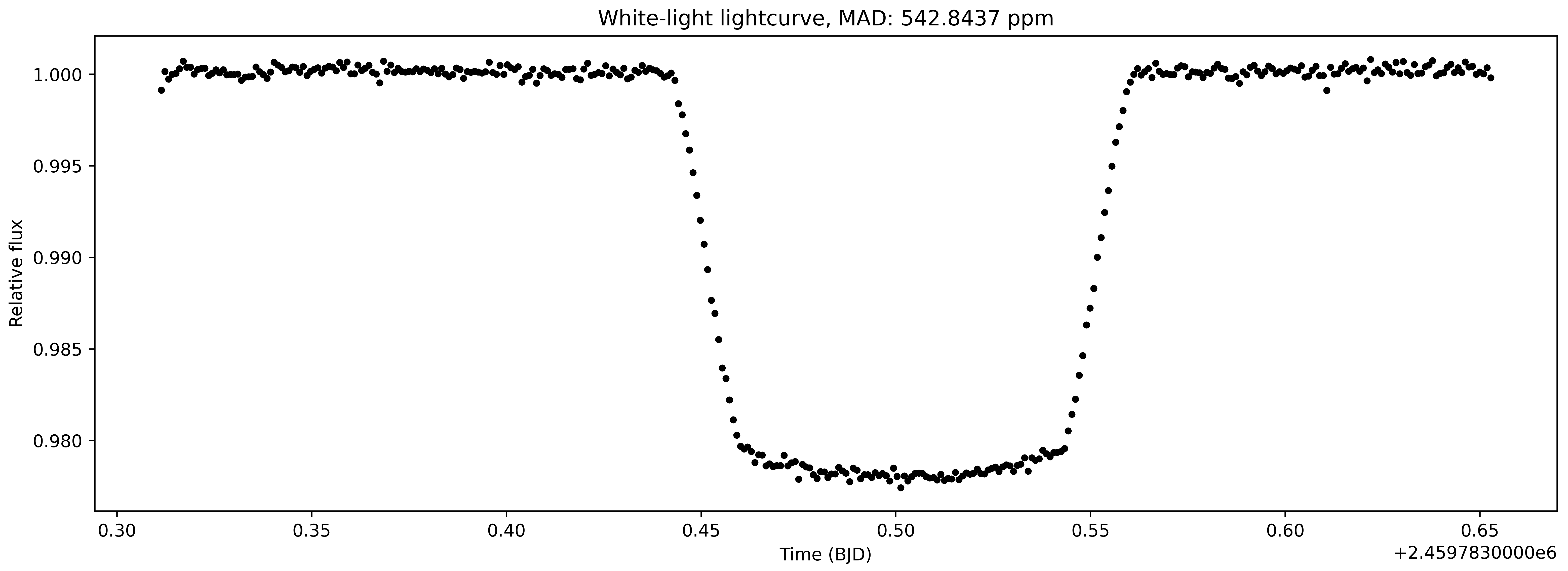
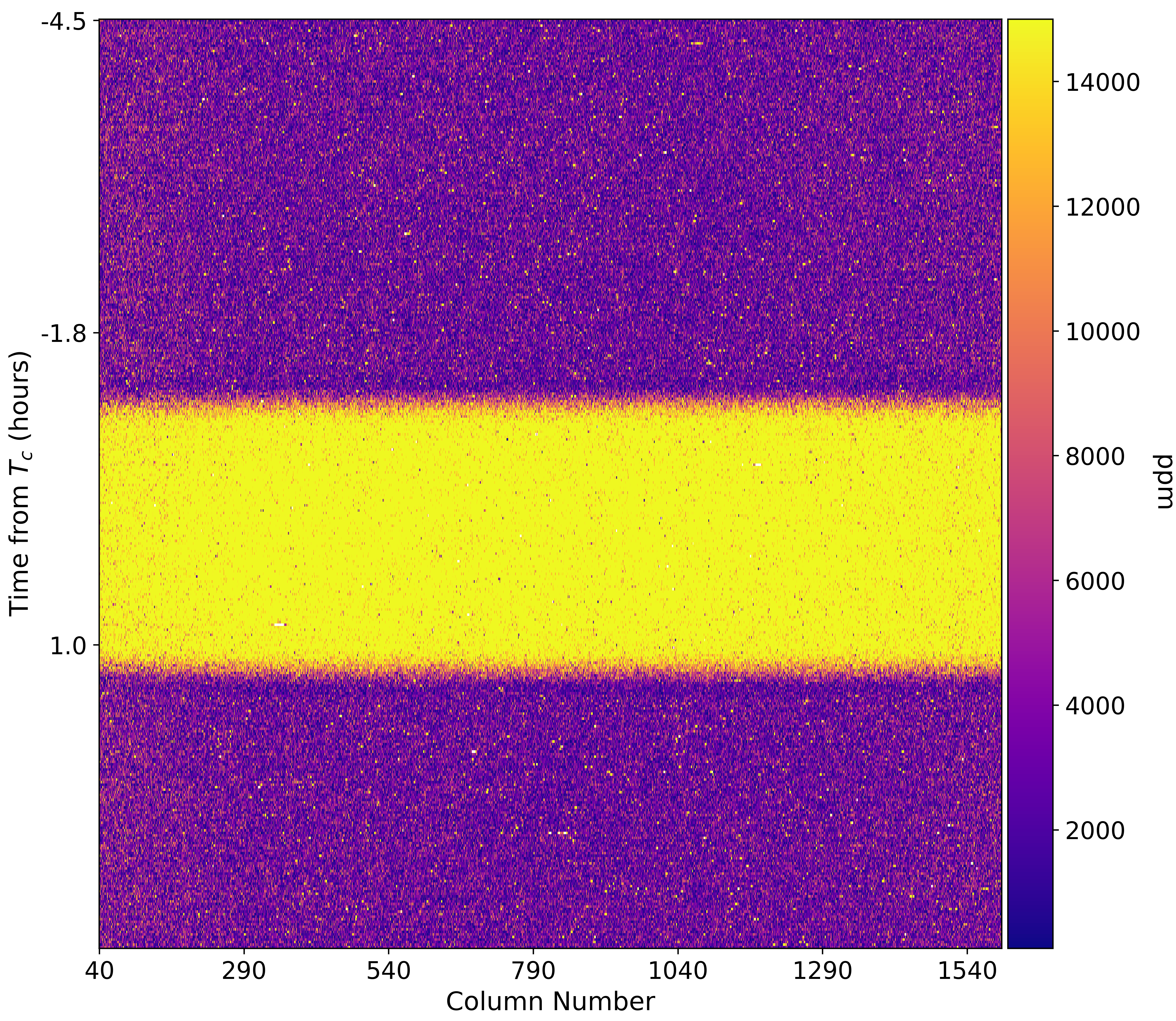
This is interesting! Probably the cleanest light curve one might have ever seen. This is a raw light curve but one cannot spot any obvious systematics. Let’s also visualise spectroscopic light curves, i.e., light curves computed for each column:

per, tc = 4.05527892, 2456401.39763
cycle = round((time_bjd[0] - tc) / per)
tc1 = tc + (cycle * per)
times_hours = (time_bjd - tc1) * 24

norm_lcs = np.zeros(spec1d.shape)
for i in range(norm_lcs.shape[1]):
    norm_lc1 = spec1d[:,i] / np.nanmedian(spec1d[:,i])
    norm_lcs[:,i] = (norm_lc1 - 1)*1e6

fig, ax1 = plt.subplots(figsize=(10, 10))

# Data
im1 = ax1.imshow(np.abs(norm_lcs), interpolation='none', cmap='plasma', aspect = 'auto')
im1.set_clim(100,15000)
plt.xlabel('Column Number', fontsize = 15)
plt.ylabel('Time from $T_c$ (hours)', fontsize = 15)

# X axis:
ticks = np.arange(0, len(xpos), 250)
ticklabels = ["{:0.0f}".format(xpos[i]) for i in ticks]
ax1.set_xticks(ticks)
ax1.set_xticklabels(ticklabels, fontsize=14)

# Y axis:
ticks = np.arange(0, len(time_bjd), 123)
ticklabels = ["{:.1f}".format(times_hours[i]) for i in ticks]
ax1.set_yticks(ticks)
ax1.set_yticklabels(ticklabels, fontsize=14)

# Colorbar:
divider = make_axes_locatable(ax1)
cax = divider.append_axes("right", size="5%", pad=0.05)

cbar = fig.colorbar(im1, shrink = 0.08, cax=cax)
cbar.ax.tick_params(labelsize=14)
cbar.ax.get_yaxis().labelpad = 20
cbar.ax.set_ylabel('ppm', rotation=270, fontsize = 15)

plt.savefig('2dtrans_spec.png', dpi=500)