Spectral extraction of a single order spectrum

In this notebook, we will extract a stellar spectrum from a single order non-timeseries data from Phoenix instrument on Gemini (South) telescope. It is a low resolution spectrograph. The data is taken on October 5, 2009 for WASP-7 and downloaded from Gemini archive. The specific data file used for this tutorial can be downloaded from here.

The data is already reduced in the sense that it is corrected for dark current and flat fielding. However, we will perform a background subtraction and correcting for 0s and NaN before extracting the spectrum.

import numpy as np
import matplotlib.pyplot as plt
from stark import SingleOrderPSF, optimal_extract, reduce, aperture_extract
from astropy.stats import mad_std
from astropy.io import fits
from tqdm import tqdm
from scipy.optimize import curve_fit as cft
from scipy.ndimage import median_filter

Loading the dataset

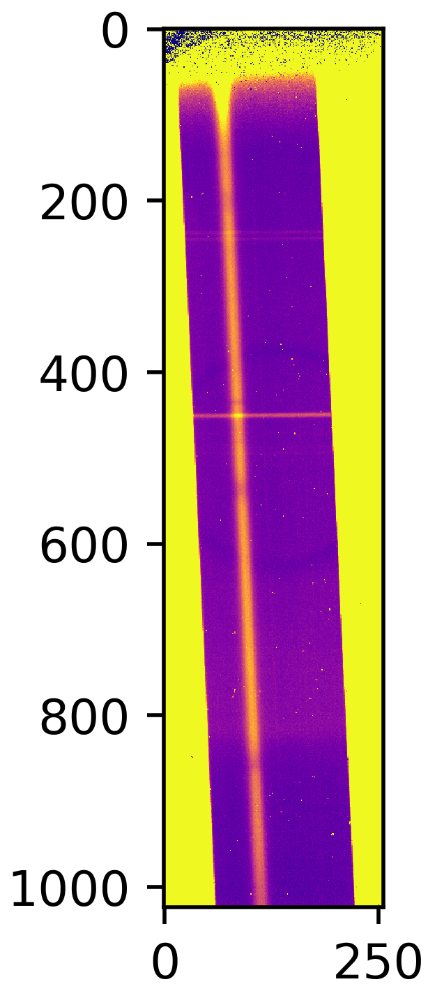
Let’s first load the data. The data is a single frame containting the flux, uncertainties and bad-pixel map. However, the default bad-pixel map that they provide is “bad” itself, so we will generate a bad-pixel map ourselvs. Let’s first visualise the data:

hdul = fits.open('2009oct25_0007_corr.fits')
data, error = hdul[0].data, hdul[2].data

plt.figure(figsize=(5/1.5,15/1.5))
im = plt.imshow(data, interpolation='none', cmap='plasma')
im.set_clim([0,100])
plt.title('The data frame')

Correcting the data and background subtraction

Good! So, we can clearly see the spectrum – note that the dispersion direction is vertical. So, we have to rotate the dataframe, since :code:`stark` assumes that the dispersion direction is horizontal, i.e., along the rows. The yellow region near the edge is the region outside of the slit. We will neglect/mask that region throughout our analysis.

Our first business is to get rid of all NaN snd 0s from the error array as they can mess up things! We will make a bad-pixel map with these pixels containing either 0 or NaN in error array.

We then want to perform a background subtraction, but looks like the trace is not perpendicular to the row/column. So, it is hard to determine background region here. What we will do is, we will first trace the location of the spectrum using centre of flux method, and then we can say that all pixels that are N pixels away from the trace are background pixels.

# Rotating the data and error frame -----
data, error = np.transpose(data), np.transpose(error)

## Correct errorbars -------
print('>>>> --- Correcting errorbars (for zeros and NaNs)...')
med_err = np.nanmedian(error.flatten())
## Changing Nan's and zeros in error array with median error
corr_err1 = np.copy(error)
corr_err2 = np.where(error != 0., corr_err1, med_err)
corrected_errs = np.where(np.isnan(error) != True, corr_err2, med_err)
print('>>>> --- Done!!')

print('>>>> --- Updating the bad-pixel map...')
## Making a bad-pixel map (1s are good pixels, 0s are bad pixels)
mask_bp1 = np.ones(data.shape)
mask_bp2 = np.where(error != 0., mask_bp1, 0.)               # This will place 0 in mask where errorbar == 0
mask_badpix = np.where(np.isnan(error) != True, mask_bp2, 0.)   # This will place 0 in mask where errorbar is Nan
print('>>>> --- Done!!')

# Visualising the spectrum
plt.figure(figsize=(15,5))
im = plt.imshow(mask_badpix, interpolation='none', cmap='plasma')
plt.title('Bad pixel map')

# Tracing the spectrum ------
def line(x, m, c):
    return m*x + c

# Finding trace
def trace_pos(data, xstart, xend, ystart, yend):
    """Given a data frame and starting location, this function will find trace
    by fitting a line to the finding maximum along the row in the dataset"""
    xpos = np.arange(xstart, xend, 1)
    trace1 = np.argmax(data[ystart:yend,xstart:xend], axis=0)
    # Fitting a linear function to this
    popt, _ = cft(line, xpos, trace1)
    median_trace = line(xpos, *popt)
    return xpos, median_trace + ystart

xpos, trace = trace_pos(data, 100, 1000, 60, 150)

# Visualising the spectrum
plt.figure(figsize=(15,5))
im = plt.imshow(data, interpolation='none', cmap='plasma')
plt.plot(xpos, trace, 'k-', lw=2.)
im.set_clim([0,100])
plt.title('The data frame with the location of the trace')

>>>> --- Correcting errorbars (for zeros and NaNs)...
>>>> --- Done!!
>>>> --- Updating the bad-pixel map...
>>>> --- Done!!

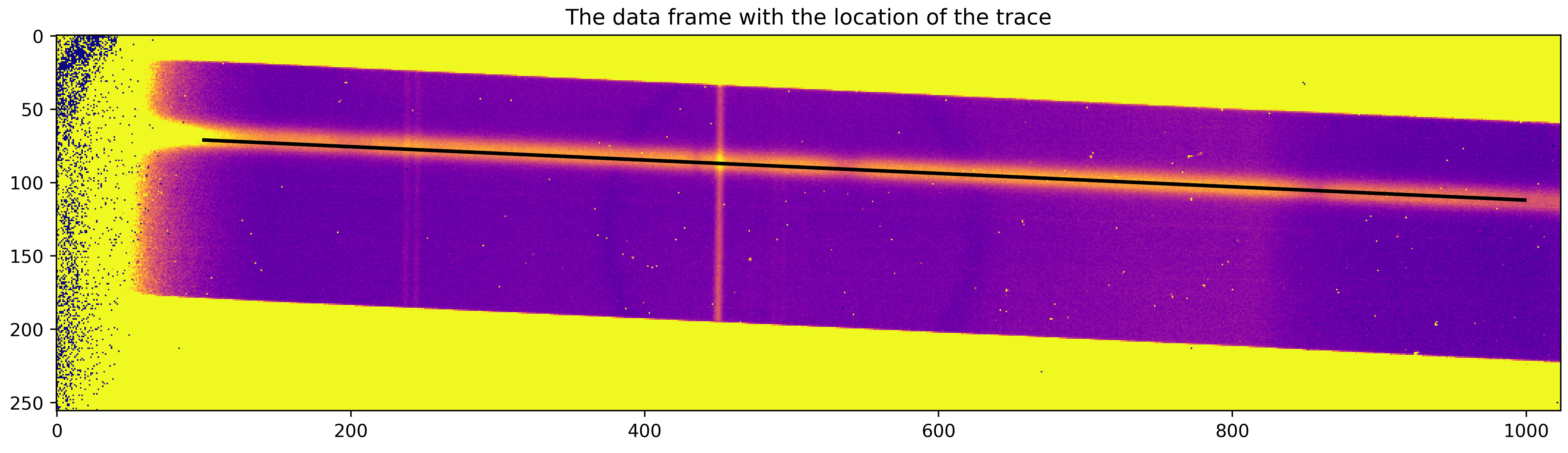
Okay, we can now determine the background region as all pixels that are at least 20 pixels away from the trace in both direction and at maximum 45 pixels away to the “above” side and 100 pixels away to the “down” side (note that the trace in not in the middle).

idx_arr_r, _ = np.meshgrid(np.arange(data.shape[0]), np.arange(data.shape[1]))
idx_arr_r = np.transpose(idx_arr_r)

dist_from_trace = np.zeros(data.shape)
dist_from_trace[:, 100:1000] = idx_arr_r[:, 100:1000]-trace[None,:]

bkg_msk = np.zeros(data.shape)
bkg_msk[(dist_from_trace > 20)&(dist_from_trace<100)] = 1.
bkg_msk[(dist_from_trace<-20)&(dist_from_trace>-45)]=1.

plt.figure(figsize=(15,5))
im2 = plt.imshow(data, interpolation='none', cmap='plasma', zorder=0)
im = plt.imshow(bkg_msk, interpolation='none', alpha=0.5, zorder=10)#, cmap='plasma')
plt.plot(xpos, trace, 'k-', lw=2.)
im2.set_clim([0,100])
plt.title('Data frame, location of the trace and background region')

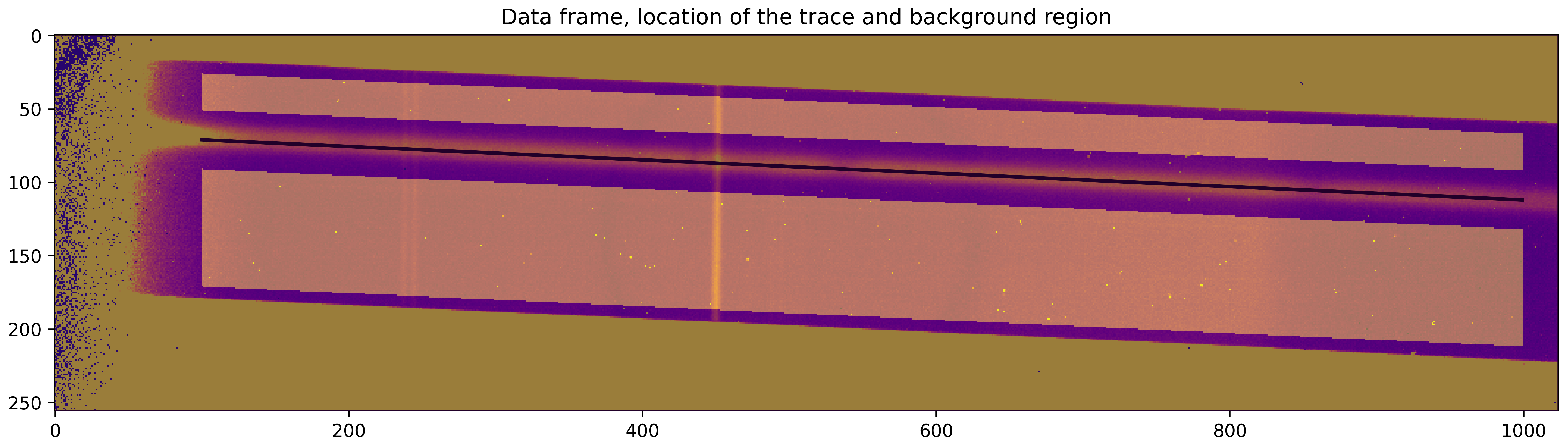
The background region is illustrated above. Let’s now perform a column-by-column background subtraction. We will fit a linear polynomial to all background pixels in a given column to estimate the background level and then subtract the estimated background from all pixels. stark has a function to do this: reduce.polynomial_bkg_cols:

bkg_corr_data, sub_image = reduce.polynomial_bkg_cols(data, bkg_msk, deg=1)

plt.figure(figsize=(15,5))
im = plt.imshow(sub_image, interpolation='none', cmap='plasma')
plt.title('Subtracted background')
im.set_clim([0,100])

Aperture extraction

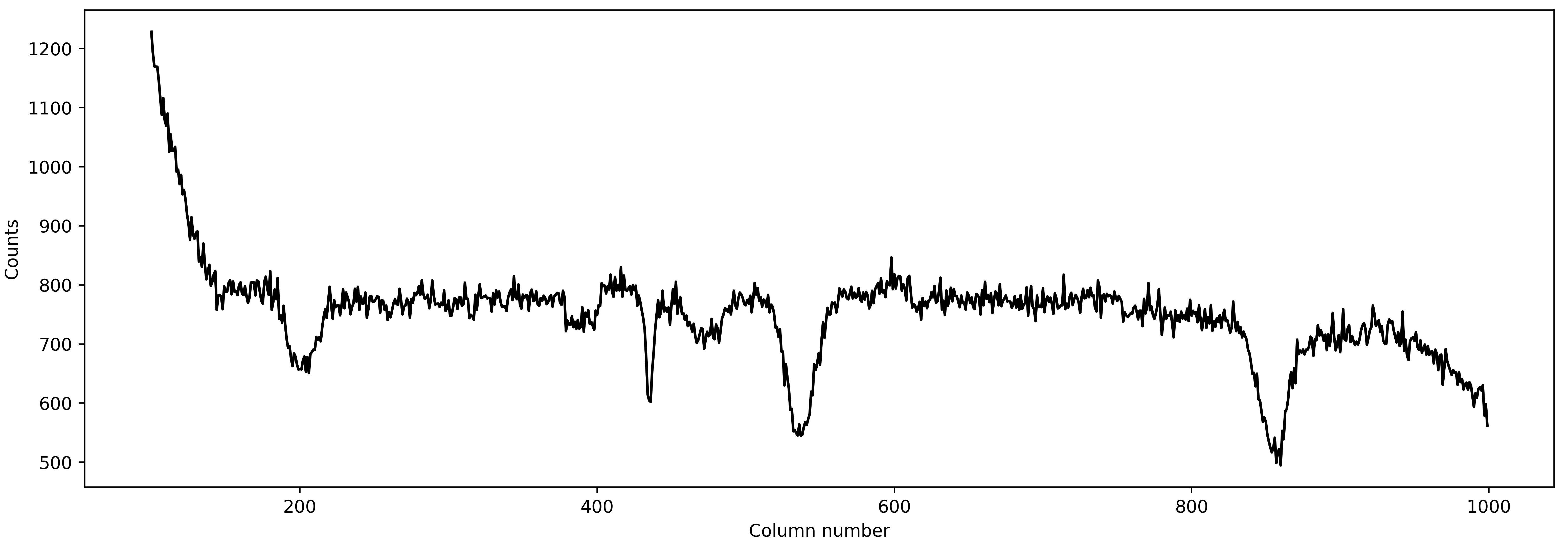
The aperture extraction, in which we simply sum up the values of flux inside the aperture to compute the spectrum, is the simplest way to estimate spectrum. However, if there are uncorrected cosmic rays (as in our case), the spectrum would have many outliers. As a first guess of the spectrum this is good enough; we will improve upon this later.

ap_extract, var_ap = aperture_extract(data[:,100:1000], error[:,100:1000], trace, ap_rad=5)

plt.figure(figsize=(15, 5))
plt.plot(xpos, ap_extract, 'k-')
plt.xlabel('Column number')
plt.ylabel('Counts')

There are some outlier columns, mostly because of uncorrected cosmic rays. We can identify t hose columns by performing a sigma clipping using a median filter. We will then replace flux values in those columns by median of neighbouring pixels.

The reason for doing so is that this spectrum will be used as a normalising spectrum below before doing the spline fitting. Now, if we do not correct for those very-high-flux cosmic ray events then the flux and variance values in the normalised data will be abnormally low. A small variance means a high weighting given to those points, which is, of course, not correct.

# Median filter of the aperture extraction (we can make the window small, because the cosmics
# usually affect only single column)
med_filt_spec = median_filter(ap_extract, size=3)

# Using 5 sigma clipping to find outliers
resids = ap_extract - med_filt_spec
limit = np.nanmedian(resids) + (10 * mad_std(resids))
msk_outliers = np.abs(resids) < limit

plt.figure(figsize=(15, 5))
plt.plot(xpos, ap_extract, 'k-', label='Aperture extraction')
plt.errorbar(xpos[~msk_outliers], ap_extract[~msk_outliers], fmt='.', c='orangered', label='Outliers')
plt.plot(xpos, med_filt_spec, 'darkgreen', label='Median filter')
plt.xlabel('Column number')
plt.ylabel('Counts')
plt.legend(loc='best')

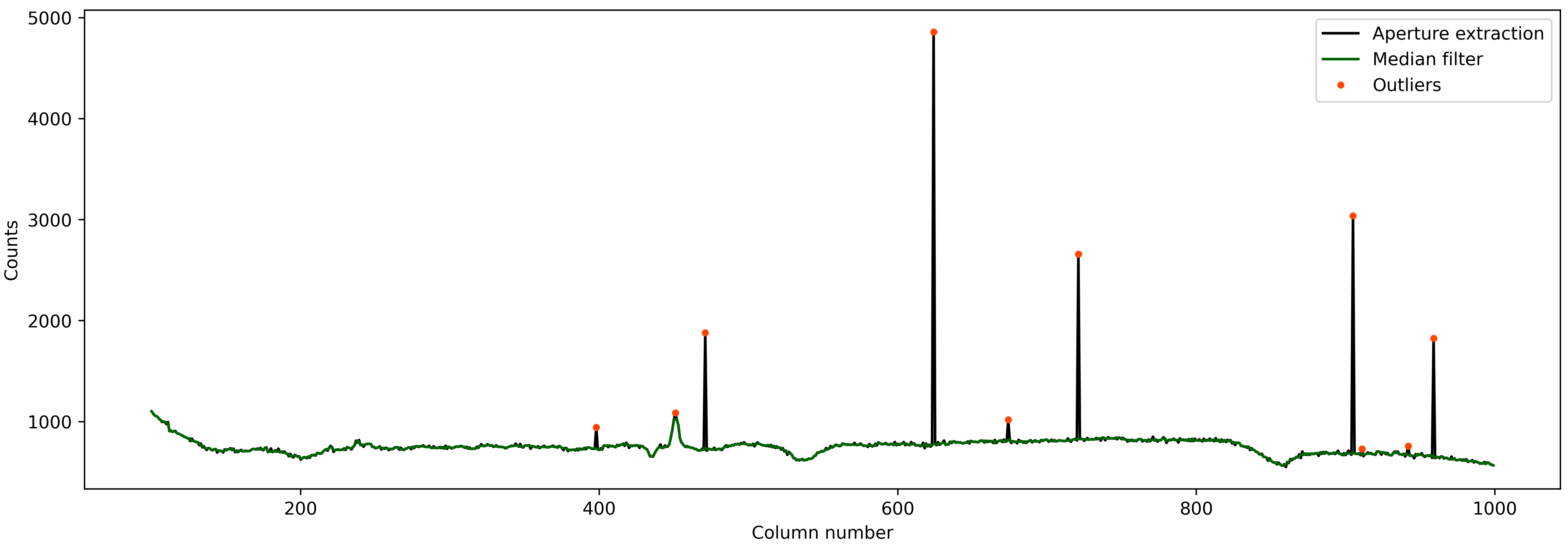
Good! Almost all bad points are identified. What we can do now is replace the value of these bad points with a median of neighbouring pixels.

ap_extract_corrected = np.copy(ap_extract)

for i in range(len(xpos)):
    if ~msk_outliers[i]:
        neigh = np.array([ap_extract[i-2], ap_extract[i-1], ap_extract[i+1], ap_extract[i+2]])
        ap_extract_corrected[i] = np.nanmedian(neigh)


plt.figure(figsize=(15, 5))
plt.plot(xpos, ap_extract, 'k-', label='Simple aperture extraction')
plt.plot(xpos, ap_extract_corrected, 'r-', label='Corrected aperture extraction')
plt.xlabel('Column number')
plt.ylabel('Counts')
plt.legend(loc='best')

Nice! We will use this corrected spectrum in our analysis now.

Initial estimate of PSF: fitting a 1D spline

We will fit a 1D spline as a function of pixel coordinate (i.e., distance from the trace) to all data within the aperture. This should give us an initial estimate of the stellar PSF. In this process of fitting a 1D spline to the data, we can even identify “bad” pixels which are affected by cosmic rays with sigma clipping. We can then mask these points in our subsequent reduction.

By default, stark assumes that the data provided to SingleOrderPSF is a timeseries data with (ntimes, nrows, ncolumns) dimension. So, since our data is only a 2D frame data and not a timeseries data, we will re-shape our data products to make them “timeseries” with only one frame in it.

# Converting 2D frames to 3D timeseries
data1 = bkg_corr_data.reshape(1, 256, 1024)
err1 = corrected_errs.reshape(1, 256, 1024)
ypos2d = trace.reshape(1,len(trace))
corr_ap_ext = ap_extract_corrected.reshape(1,len(ap_extract_corrected))
mask_badpix = mask_badpix.reshape(1, 256, 1024)

# And fitting a 1D spline
data1d = SingleOrderPSF(frame=data1[:,:,xpos[0]:xpos[-1]+1],\
                        variance=err1[:,:,xpos[0]:xpos[-1]+1]**2,\
                        mask=mask_badpix[:,:,xpos[0]:xpos[-1]+1],\
                        ord_pos=ypos2d, ap_rad=15., spec=corr_ap_ext)
psf_frame1d, psf_spline1d, msk_updated_1d = data1d.univariate_psf_frame(niters=5, oversample=1, clip=5)

ts1 = np.linspace(np.min(data1d.norm_array[:,0]), np.max(data1d.norm_array[:,0]), 1000)
msk1 = np.asarray(data1d.norm_array[:,4], dtype=bool) * msk_updated_1d
plt.figure(figsize=(16/1.5, 9/1.5))
plt.errorbar(data1d.norm_array[msk1,0], data1d.norm_array[msk1,1], fmt='.')
plt.plot(ts1, psf_spline1d(ts1), c='k', lw=2., zorder=10)
plt.xlabel('Distance from the trace')
plt.ylabel('Normalised flux')

Iter 1 / 5: 0.04659 per cent masked.
Iter 2 / 5: 0.08244 per cent masked.
Iter 3 / 5: 0.08244 per cent masked.
Iter 4 / 5: 0.08244 per cent masked.
Iter 5 / 5: 0.08244 per cent masked.

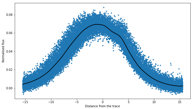
I think this is very good PSF fitting (in black) for a first estimate. As can be seen, the PSF is very broad.

One of the products of SingleOrderPSF.univariate_psf_frame is a mask containing all points discarded while performing sigma clipping during spline fiting. This mask is not in a format of 2D frame but rather in a form of “pixel table”. The “pixel table” is an internal method to store data products. stark has a function to convert the data from this “pixel table” to 2D frames that we can understand. We will add the points in this mask to our bad pixel map and will not include in our further reduction.

msk_2d = data1d.table2frame(msk_updated_1d)
mask_badpix_updated = np.copy(mask_badpix)
mask_badpix_updated[:,:,xpos[0]:xpos[-1]+1] = mask_badpix[:,:,xpos[0]:xpos[-1]+1] * msk_2d

plt.figure(figsize=(15,5))
plt.imshow(mask_badpix_updated[0,:,:], interpolation='none', cmap='plasma')
plt.title('Updated bad-pixel map')

And now, we will use this updated bad-pixel map to extract the spectrum below:

(Again, altogh there is only one frame in our data, we will continue to consider it as a “timeseries” because by default the SingleOrderPSF class assumes that the data is in timeseries.)

spec1d, var1d = np.zeros((psf_frame1d.shape[0], psf_frame1d.shape[2])), np.zeros((psf_frame1d.shape[0], psf_frame1d.shape[2]))
syth1d = np.zeros(psf_frame1d.shape)
for inte in tqdm(range(spec1d.shape[0])):
    spec1d[inte,:], var1d[inte,:], syth1d[inte,:,:] = optimal_extract(psf_frame=psf_frame1d[inte,:,:],\
                                                                    data=data1[inte,:,xpos[0]:xpos[-1]+1],\
                                                                    variance=err1[inte,:,xpos[0]:xpos[-1]+1]**2,\
                                                                    mask=mask_badpix_updated[inte,:,xpos[0]:xpos[-1]+1],\
                                                                    ord_pos=ypos2d[inte,:], ap_rad=15.)

spec_from1d = spec1d[0,:]
plt.figure(figsize=(15, 5))
plt.plot(xpos, spec1d[0,:], 'k-')
plt.xlabel('Column number')
plt.ylabel('Counts')

A good spectrum with almost no outliers! This is great! We can now use this spectrum and go for an estimation of even more robust PSF by fitting a 2D spline to the data.

Robust estimate of the PSF: fitting a 2D spline

While fitting a 1D spline only as function of pixel coordinates can give a good estimate of the stellar PSF (and, the spectrum, subsequently), it may be a poor estimate of the PSF. The main assumption while fitting a 1D spline to the data is that the stellar PSF does not change with wavelength. This is, however, not true: the PSF changes significantly with wavelength. Therefore, we will fit a 2D spline to the data as a function of pixel-coordinate (i.e., distance from the trace) and wavelength. We will use the better estimate of stellar spectrum found above as a normalising constant in preparing the data.

data2 = SingleOrderPSF(frame=data1[:,:,xpos[0]:xpos[-1]+1],\
                       variance=err1[:,:,xpos[0]:xpos[-1]+1]**2,\
                       ord_pos=ypos2d, ap_rad=15., mask=mask_badpix_updated[:,:,xpos[0]:xpos[-1]+1],\
                       spec=spec1d)
psf_frame2d, psf_spline2d, msk_after2d = data2.bivariate_psf_frame(niters=3, oversample=2, knot_col=10, clip=5)

/Users/japa6985/opt/anaconda3/envs/jwst/lib/python3.9/site-packages/scipy/interpolate/fitpack2.py:1272: UserWarning:
The coefficients of the spline returned have been computed as the
minimal norm least-squares solution of a (numerically) rank deficient
system (deficiency=62). If deficiency is large, the results may be
inaccurate. Deficiency may strongly depend on the value of eps.
warnings.warn(message)
Iter 1 / 3: 0.09677 per cent masked.
Iter 2 / 3: 0.09677 per cent masked.
Iter 3 / 3: 0.09677 per cent masked.

First, let’s see how the best fitted PSF looks for an arbitrary column

# Details are not that important:
# But what we are trying to do below is to find data from an arbitrary column for _all_ integration
# And then we will see how the fitted 2D spline behaves to this data

ncol1 = np.random.choice(xpos)  # Arbitrary column number
msk5 = data2.col_array_pos[:,ncol1,0]     # Mask data
npix1 = data2.col_array_pos[:,ncol1,1]    # Pixel radius data

xpoints = np.array([])     # To save x (pixel coordinate), y (column no), z (flux)
ypoints = np.array([])
zpoints = np.array([])
for i in range(len(msk5)):
    xdts = data2.norm_array[msk5[i]:msk5[i]+npix1[i],0]
    ydts = data2.norm_array[msk5[i]:msk5[i]+npix1[i],3]
    zdts = data2.norm_array[msk5[i]:msk5[i]+npix1[i],1]
    msk_bad = np.asarray(data2.norm_array[msk5[i]:msk5[i]+npix1[i],4], dtype=bool)
    xdts, ydts, zdts = xdts[msk_bad], ydts[msk_bad], zdts[msk_bad]
    xpoints = np.hstack((xpoints, xdts))
    ypoints = np.hstack((ypoints, ydts))
    zpoints = np.hstack((zpoints, zdts))

# Creating a continuous grid of points
xpts1 = np.linspace(np.min(xpoints)-0.1, np.max(xpoints)+0.1, 1000)
ypts1 = np.ones(1000)*ypoints[0]

fits_2d = psf_spline2d(xpts1, ypts1, grid=False)

plt.figure(figsize=(16/1.5,9/1.5))
plt.errorbar(xpoints, zpoints, fmt='.')
plt.plot(xpts1, fits_2d, 'k-')
plt.plot(xpoints, psf_spline2d(xpoints, ypoints, grid=False), 'k.')
plt.axvline(0., color='k', ls='--')
plt.title('For Column ' + str(ncol1))
plt.xlabel('Distance from the trace')
plt.ylabel('Normalised flux')

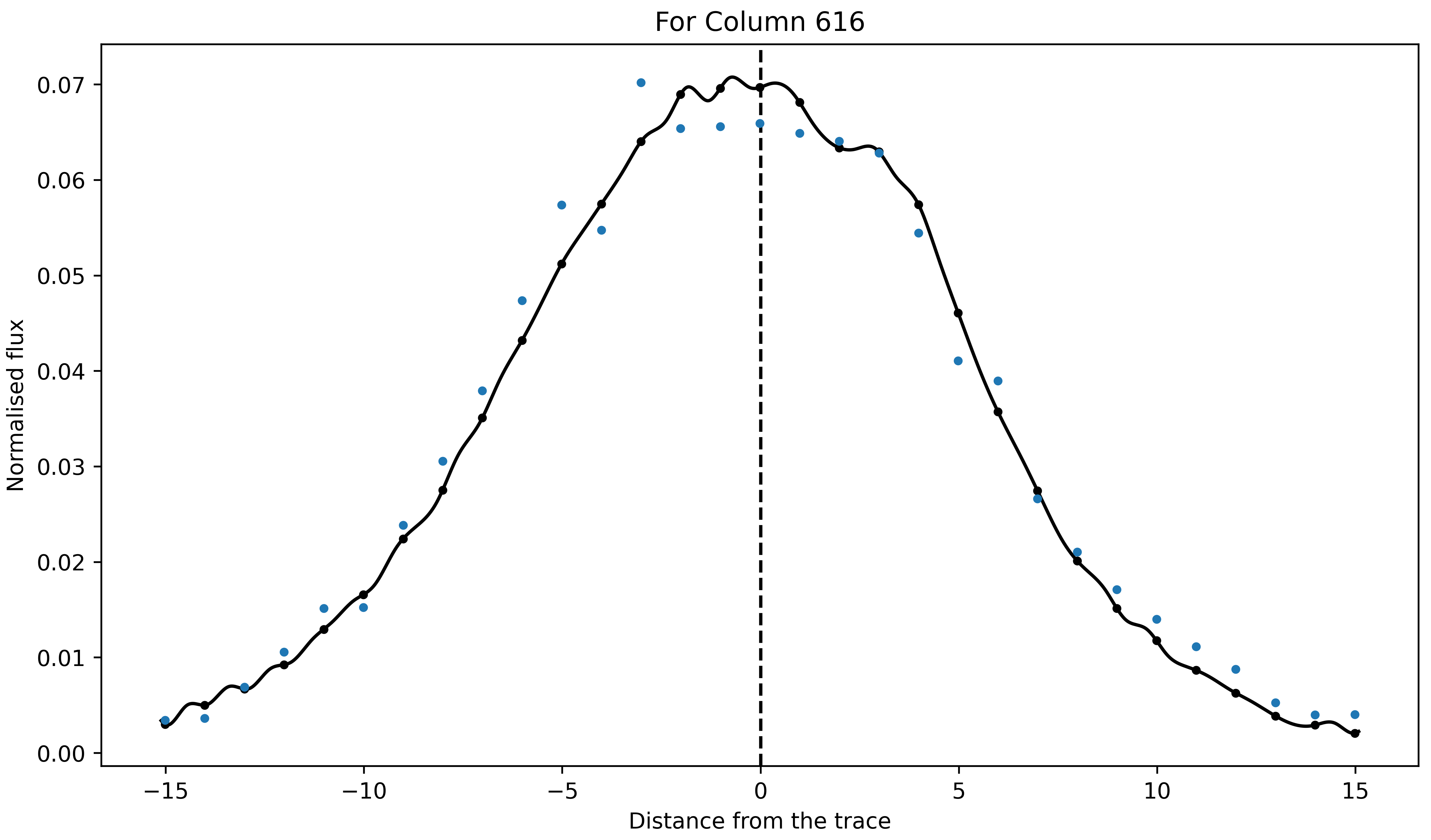
Not bad! We above mentioned that the PSF will change with wavelength. Let’s now see if this is indeed the case or not by computing amplitude and FWHM of the best-fitted PSF as a function of wavelength:

# Defining pixel coordinates
pix_cor_res = 50000
pix_corr = np.linspace(-8., 8., pix_cor_res)

cols = xpos - xpos[0]
max_amp = np.zeros(len(cols))
fwhm = np.zeros(len(cols))

for i in range(len(cols)):
    fit2 = psf_spline2d(x=pix_corr, y=np.ones(pix_cor_res)*cols[i], grid=False)
    # Maximum amplitude
    max_amp[i] = np.max(fit2)
    # Maximum amplitude location
    idx_max_amp = np.where(fit2 == np.max(fit2))[0][0]
    # fwhm
    hm = (np.max(fit2) + np.min(fit2))/2
    idx_hm = np.where(np.abs(fit2 - hm)<0.005)[0]
    idx_hm_up, idx_hm_lo = 0, 0
    diff_up1, diff_lo1 = 10., 10.
    for j in range(len(idx_hm)):
        if idx_hm[j] > idx_max_amp:
            diff_u1 = np.abs(fit2[idx_hm[j]] - hm)
            if diff_u1 < diff_up1:
                diff_up1 = diff_u1
                idx_hm_up = idx_hm[j]
        else:
            diff_l1 = np.abs(fit2[idx_hm[j]] - hm)
            if diff_l1 < diff_lo1:
                diff_lo1 = diff_l1
                idx_hm_lo = idx_hm[j]
    fwhm[i] = np.abs(pix_corr[idx_hm_up] - pix_corr[idx_hm_lo])

fig, axs = plt.subplots(2, 1, figsize=(15, 5), sharex=True, facecolor='white')

axs[0].plot(xpos, max_amp, 'k-')
axs[0].set_ylabel('Maximum Amplitude', fontsize=14)

axs[1].plot(xpos, fwhm, 'k-')
axs[1].set_ylabel('FWHM', fontsize=14)
axs[1].set_xlabel('Column number', fontsize=14)

axs[1].set_xlim([xpos[0], xpos[-1]])

axs[0].set_title('PSF evolution with wavelength', fontsize=15)

plt.setp(axs[0].get_yticklabels(), fontsize=12)
plt.setp(axs[1].get_xticklabels(), fontsize=12)
plt.setp(axs[1].get_yticklabels(), fontsize=12)

plt.tight_layout()

Aha! So, the PSF does change with wavelength. As can be seen, the FWHM of the PSF decreases significantlly with the wavelength (i.e., with column number). This is why fitting 1D spline without taking into account the wavelength information would give a poor estimate of the stellar PSF, and hence, the stellar spectrum. We will now use this robust estimate of the PSF to compute the spectrum. But before doing that, first, let’s update the bad pixel map.

Similar to the univariate_psf_frame, bivariate_psf_frame also returns a mask in the format of pixel table as described above. We can update the mask as follows:

msk_2d2d = data2.table2frame(msk_after2d)
mask_badpix_updated2d = np.copy(mask_badpix_updated)
mask_badpix_updated2d[:,:,xpos[0]:xpos[-1]+1] = mask_badpix_updated[:,:,xpos[0]:xpos[-1]+1] * msk_2d2d

plt.figure(figsize=(15,5))
plt.imshow(mask_badpix_updated2d[0,:,:], interpolation='none', cmap='plasma')
plt.title('Updated bad-pixel map')

And, now the spectrum,

spec1d, var1d = np.zeros((psf_frame2d.shape[0], psf_frame2d.shape[2])), np.zeros((psf_frame2d.shape[0], psf_frame2d.shape[2]))
syth1d = np.zeros(psf_frame2d.shape)
for inte in tqdm(range(spec1d.shape[0])):
    spec1d[inte,:], var1d[inte,:], syth1d[inte,:,:] = optimal_extract(psf_frame=psf_frame2d[inte,:,:],\
                                                                    data=data1[inte,:,xpos[0]:xpos[-1]+1],\
                                                                    variance=err1[inte,:,xpos[0]:xpos[-1]+1]**2,\
                                                                    mask=mask_badpix_updated2d[inte,:,xpos[0]:xpos[-1]+1],\
                                                                    ord_pos=ypos2d[inte,:], ap_rad=15)

spec_from2d = spec1d[0,:]
plt.figure(figsize=(15, 5))
plt.plot(xpos, spec1d[0,:], 'k-')
plt.xlabel('Column number')
plt.ylabel('Counts')

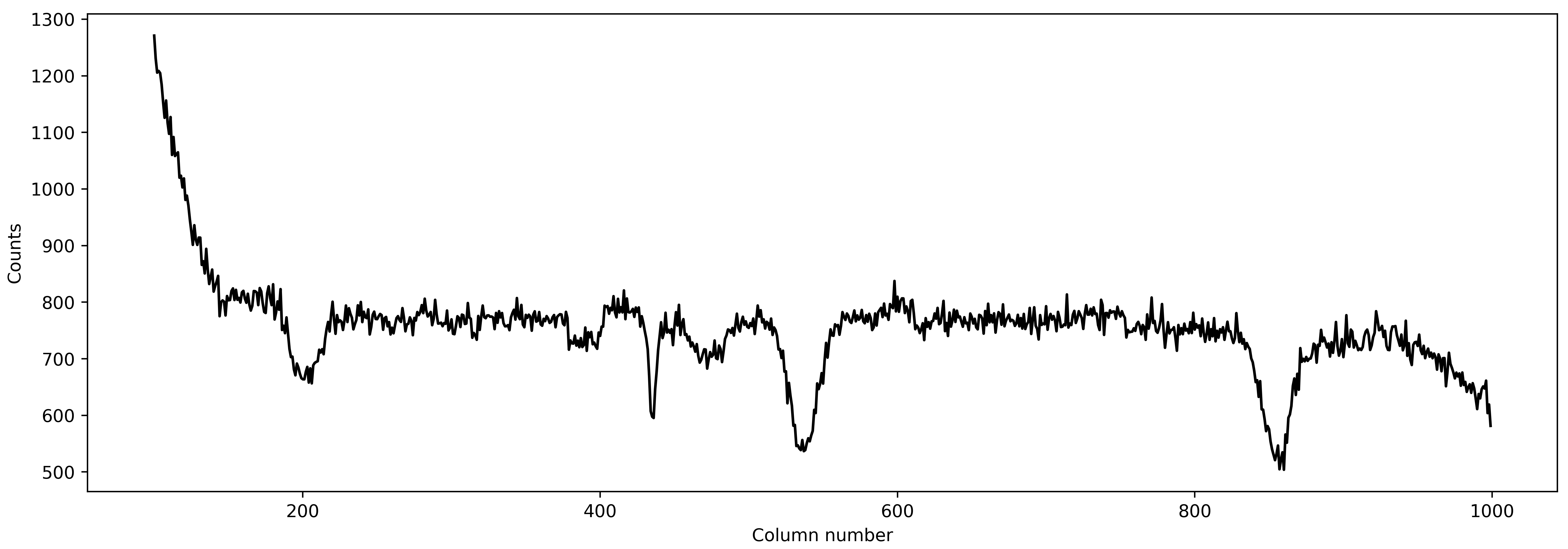
Fantastic! Let’s see how the spectrum changed from aperture extraction to this more robust extraction:

plt.figure(figsize=(15, 5))
plt.plot(xpos, ap_extract_corrected, 'k-', label='Aperture extraction')
plt.plot(xpos, spec_from1d, color='orangered', label='1D spline extraction')
plt.plot(xpos, spec_from2d, color='dodgerblue', label='2D spline extraction')
plt.xlabel('Column number')
plt.ylabel('Counts')
plt.legend(loc='best')

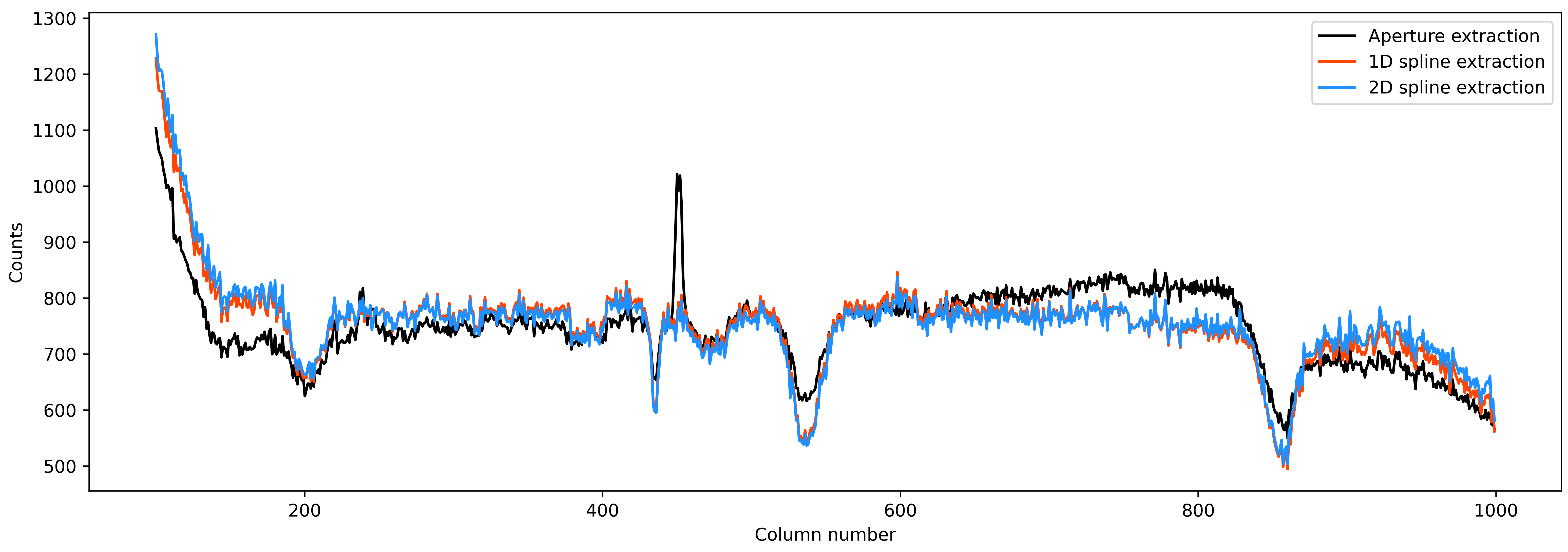
Nice! Finally, as a reduction diagnostic, let’s have a look at the residual frame.

The optimal_extract function, in addition to the spectrum and variance, also returns a sythetic data frame. This frame is constructed from the estimate of PSF and the stellar spectrum. We can subtract this frame from the data frame and look for any remaining structures in the resultant residual frame. Any significant remaining structures in the residual frames indicates that the PSF fitting and extraction was not optimal.

resid = np.zeros(syth1d.shape)
resid[0,:,:] = data1[0,:,xpos[0]:xpos[-1]+1] - syth1d[0,:,:]

plt.figure(figsize=(15,5))
im = plt.imshow(resid[0,:,:], interpolation='none', cmap='plasma')
#plt.plot(xpos-xpos[0], trace, 'k-', lw=0.5)
plt.plot(xpos-xpos[0], trace+15, 'k--', lw=.5)
plt.plot(xpos-xpos[0], trace-15, 'k--', lw=.5)
im.set_clim([-10,10])
plt.title('Residual frame')

The two lines shows the extent of apeture and thus extent of our extraction. We want to look for any obvious structures inside the aperture. It appears that there is no significant structures inside the aperture. The big circular thing (which was also present in the data frame above, but not visible due to color limits) is an effect of the flat fielding. Except for that, there is no significant structures in the residuals demonstrating the quality of our extraction.